Installation
cisTEM is optimized to run on CPUs; GPUs are currently not supported. It has its own parallelization scheme that is independent of common architectures such as openMPI. Furthermore, it can run on a local workstation and utilize high-performance computing environments (e.g. a computer cluster) by remotely executing compute jobs. All that is required is that all machines (local workstation, cluster login and compute nodes) have access to the same file system (i.e. paths to data files and the cisTEM installation directory are the same everywhere) and, in case a cluster is used, that the login node is accessible via ssh.
To install cisTEM, download one of the precompiled versions of cisTEM to take advantage of optimizations that may not be available when compiling on a local machine. Select the archive that is appropriate for the architecture used and, after downloading it to a local disk, unpack it using the command line
tar -xzf cistem-<version>-<architecture>-<OS>.tar.gz
This will create a directory called cistem-<version> that contains all the necessary programs to run cisTEM. Type the command line
cistem-<version>/cisTEM
This should start the cisTEM graphical user interface (GUI), indicating that cisTEM is able to run on your system. Close the cisTEM windows and finish the installation by including the cistem-<version> directory in your PATH environment variable for executables. Then, after logging out and back in, you should be able to start cisTEM by typing
cisTEM
on the command line. If everything was installed correctly, this will start the cisTEM GUI. To run cisTEM on a computer cluster or remote machines, it wil also be necessary to add or edit Run Profiles that can be managed on the Settings panel.
Getting Started & Tutorial
The best way to become familiar with cisTEM is to work through the tutorial, which starts with movies of apoferritin and takes the user all the way to a 3-Å reconstruction. The dataset contains 20 movies, stored in MRC format, the default format for all cisTEM image data. The size of the dataset is modest, enabling completion of the tutorial in just a few hours on most computer systems. The final result of the tutorial, a 3-Å reconstruction, is also attached below, as well as a comprehensive publication describing more technical aspects of cisTEM.
To start a new project, launch cisTEM and click on the Create a new project link on the Overview panel shown on startup. A dialog allows the user to define a project name and a path when a directory with the name of the project is created. This directory contains all project-related files, including intermediate and final class averages and reconstructions.
Once a new project is created, different types of Assets can be imported, for example, movies or micrographs (images). Actions can then be used to process Assets and produce Results, often resulting in new Assets of a different type. The different cisTEM panels are described in more detail on the Assets, Actions and Results Panel documentation pages.
Apoferritin Tutorial Dataset
|
Parameter |
Value |
|---|---|
|
Beam energy (keV) |
300 |
|
Spherical aberration (mm) |
0.0 |
|
Pixel size (Å) |
1.5 |
|
Exposure rate (el/Å2/frame) |
2.0 |
|
Molecular mass (kDa) |
440 |
|
Largest dimension (Å) |
120 |
|
Symmetry |
O |
If the download link for apoferritin_data.tar.gz below does not work or the download does not complete, the tutorial dataset can also be downloaded from the EMPIAR database.
![]() cisTEM_tutorial.pdf
cisTEM_tutorial.pdf![]() Grant_eLife2018.pdf
Grant_eLife2018.pdf![]() apoferritin.mrc
apoferritin.mrc![]() apoferritin_data.tar.gz
apoferritin_data.tar.gz
Movie & Image Assets
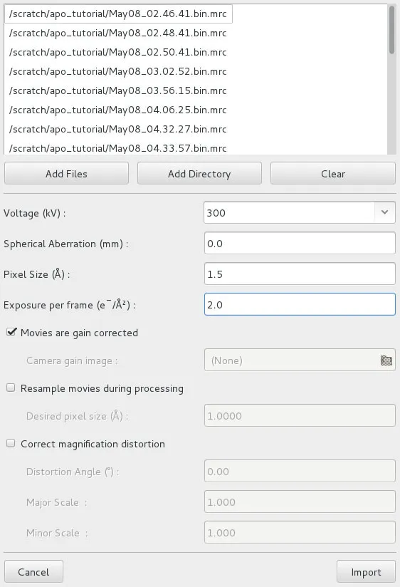
Once a project is open or has been newly created, Movies or Images can be imported. Image Assets can also be generated by processing Movies (see Align Movies Actions panel). To import, click on Assets, then Movies or Images, and then Import. This will open a dialog (the figure shows a Movies import dialog).
In the dialog, select Add Files or Add Directory and navigate to the files/directory containing the Movies. Then click Open. This should list all the movies in the directory. Now enter the required information describing the data: Voltage (kV), Spherical Aberration (mm), Pixel Size (Å), and for Movies, Exposure per frame (e–/Å2). For Movies, there are also options to import compressed tiff files (as generated by SerialEM) and separate gain references, to change the pixel size (binning) and apply magnification distortion on the fly. Users should consider increasing the pixel size, for example doubling it, when importing movies/images recorded in super-resolution mode to save processing time and disk/memory space. In most cases, super-resolution will not yield higher resolution of the final reconstructions. The binning algorithm implemented in cisTEM uses Fourier cropping and should therefore not result in the loss of signal in the frequency domain of the resulting movie/image.
Click Import and cisTEM will show a list of the imported Movies/Images. The Movies/Images are all part of a group called “All Movies” or “All Images.” Additional groups can be created using Add to select subsets of a dataset for further processing. Movie and Image Assets can be renamed or removed, and added to user-defined groups (by clicking Add To Group or selecting the Asset and dragging it onto the group). They can also be displayed by clicking Display. Image Asset groups can also be defined from Movie groups by clicking New from movie group. This is useful, for example, when a subset of good movies was defined based on the CTF determination results (see Find CTF Results panel), and only the corresponding images should be included for further processing, for example, for particle selection.
Particle Position Assets
Particle Positions are Assets that identify particles in Images and are usually generated by running the Find Particles Action. However, they can also be imported from a text file listing for each particle the Asset ID of the image they belong to, the x-coordinate in Å (along the fast axis of the image pixel array) and the y-coordinate in Å (along the slow axis of the image pixel array):
0 377.52 1888.64
0 989.04 1880.32
0 1687.92 1882.4
0 157.04 1876.16
0 799.76 1824.16
0 1045.2 1826.24
0 236.08 1822.08
0 342.16 1813.76
0 400.4 1797.12
1 546 1807.52
1 708.24 1797.12
1 957.84 1807.52
1 1174.16 1797.12
1 1490.32 1822.08
1 1669.2 1813.76
1 1723.28 1772.16
2 177.84 1753.44
2 1542.32 1745.12
2 310.96 1732.64
2 589.68 1718.08
…
Instead of the Image Asset ID, the list can also contain the file name of the Asset (the attached file at the bottom of this page contains an example script written by by Matthias Wolf to convert a Relion star file with picked particle coordinates to such a list):
May08_02.46.41.bin_0_0.mrc 377.52 1888.64
May08_02.46.41.bin_1_0.mrc 989.04 1880.32
May08_02.46.41.bin_2_0.mrc 1687.92 1882.4
May08_02.46.41.bin_3_0.mrc 157.04 1876.16
May08_02.46.41.bin_4_0.mrc 799.76 1824.16
May08_02.46.41.bin_5_0.mrc 1045.2 1826.24
May08_02.46.41.bin_6_0.mrc 236.08 1822.08
May08_02.46.41.bin_7_0.mrc 342.16 1813.76
May08_02.46.41.bin_8_0.mrc 400.4 1797.12
May08_02.48.41.bin_9_0.mrc 546 1807.52
May08_02.48.41.bin_10_0.mrc 708.24 1797.12
May08_02.48.41.bin_11_0.mrc 957.84 1807.52
May08_02.48.41.bin_12_0.mrc 1174.16 1797.12
May08_02.48.41.bin_13_0.mrc 1490.32 1822.08
May08_02.48.41.bin_14_0.mrc 1669.2 1813.76
May08_02.48.41.bin_15_0.mrc 1723.28 1772.16
May08_02.50.41.bin_16_0.mrc 177.84 1753.44
May08_02.50.41.bin_17_0.mrc 1542.32 1745.12
May08_02.50.41.bin_18_0.mrc 310.96 1732.64
May08_02.50.41.bin_19_0.mrc 589.68 1718.08
…
To import Particle Positions, click on Import on the Particle Positions Asset panel and browse to the text file containing the coordinates. Then click Open.
Using Asset groups, picked particles can be divided into subgroups. This is useful, for example, when multiple particle picking jobs were run (see Find Particles Action panel) and only particles from a specific job should be used. The picking job that generated a Particle Position is listed in the “Pick Job I.D.” column.
3D Volume Assets
3D Volume Assets represent 3D density maps that are generated from Actions including Ab-Initio 3D, Auto Refine and Manual Refine. They can also be imported to be used as references in refinement jobs. To import a map, click Import on the 3D Volumes Asset panel, then Add Files and browse to the map file(s) to import, then click Open. Alternatively, whole directories can be imported by clicking Add Directory, then Open. For each import, the pixel size of the density map has to be entered. Then click Import. The pixel size must match the pixel size of the Movies/Images and Refinement Package that the 3D Volume(s) will be used with. Like other Assets, 3D Volumes can be grouped into subgroups.
Refinement Package Assets
Refinement Packages are defined by a particle image stack, a set of particle alignment parameters, and optionally a 3D Volume (or several 3D Volumes if more than one 3D class is requested, see "How do I start 3D classification?" in FAQs). Therefore, a Refinement Package contains all the information required to perform the refinement of a 3D density map. Refinement Packages can be created from Particle Positions by clicking Create. This will start a wizard to collect all the required information. In the simplest case, a new Refinement Package is created, using Particle Positions to box out particles, assemble them to a stack and assign a set of random alignment parameters to them. For the template Refinement Package, select New Refinement Package, click Next and select the set of Particle Positions to be used, for example All Positions, then Next and the desired particle box size (sufficiently large to include particle and CTF-delocalized signal), approximate molecular weight of the particle, the largest dimension in Å, the particle symmetry, and the number of desired 3D classes (see also "How do I start 3D classification?" in FAQs). The wizard will then create a particle stack and assign random parameters to each particle. The resulting Refinement Package can be used for Ab Initio 3D reconstruction, for example, or a 3D Volume can be assigned and used as an initial reference to align the particles in the stack. To assign a 3D Volume, double-click on the entry in Active 3D References and select one of the available 3D Volumes as a reference. Selecting Generate From Params. will calculate a 3D Volume from the current parameters assigned to the particles. For a new refinement package, this will result in an approximately spherical volume corresponding to the assigned random angles. However, if the Refinement Package was imported or derived from an earlier Refinement Package (see below), the 3D reconstruction corresponding to the imported/earlier parameters will be generated. The box size chosen for the Refinement Package has to match the box size of the 3D Volume. The particle stack can be displayed using the Display Stack button.
A Refinement Package can also be created from an existing Refinement Package. In this case, select one of the existing Refinement Packages from the menu as the template Refinement Package. After clicking Next, the menu provides a choice of alignment parameters that are associated with the chosen Refinement Package template. Usually, the parameters giving the best reconstruction in the previous refinement is selected here, often the last on the list. However, parameters corresponding to intermediate results can also be chosen. The selection can be changed later on when running a refinement (see Automatic/Manual Refinement). Default answers are provided to the remaining questions in the wizard, based on the template. The user can change these to achieve different goals. For example, the symmetry can be changed to either impose symmetry where there was no symmetry imposed before, or to remove symmetry and do an asymmetric refinement. The number of classes can also be changed to allow 3D classification (see "How do I start 3D classification?" in FAQs). Creating a Refinement Package in this way will not recreate the particle stack.
A third way to create a Refinement Package is based on 2D classification results (see 2D Classification). Selecting Create From 2D Class Average Selection as the template will provide a list of groups of 2D class averages that can be defined in the 2D Classification results panel. The remaining questions are the same as before, generating a particle stack and set of parameters that contain only the particles that ended up in the selected 2D class averages.
Finally, Refinement Packages can be imported from Frealign and Relion refinements. Click Import and select the type of the refinement to be imported. The import wizard will then ask for the location of the particle stack and parameter file (either a Frealign par file or a Relion Star file). Next, the relevant microscope parameters will have to be entered: pixel size, acceleration voltage, spherical aberration coefficient, amplitude contrast, symmetry, approximate molecular weight, largest dimension, and the “polarity” of the particle density in the images. The polarity for Frealign refinements is typically black particles on light background while it is white particles on dark background in Relion refinements. Click Finish to import the data. Please note that the particle stack is not copied and has to remain in place while being worked on using cisTEM. It is therefore good practice to import a copy of the particle stack that is placed in a safe location, for example inside the cisTEM project directory.
Aligning Movies
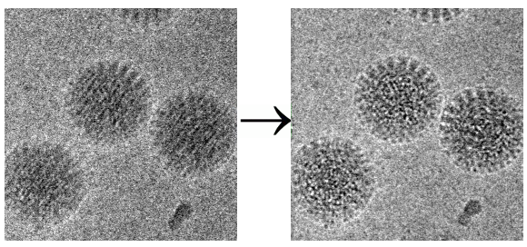
The frames of Movies can be aligned using the Align Movies Action panel. Physical drift and beam induced motion (Brilot et al., 2012; Campbell et al., 2012; Li et al., 2013; Scheres, 2014) of the specimen leads to a degradation of information within images, and will ultimately limit the resolution of any reconstruction. Aligning a movie prior to calculating the sum will prevent a large amount of this degradation and lead to better data. The Align Movies panel therefore attempts to align movies based on the Unblur algorithm described in (Grant and Grigorieff, 2015).
Additionally an exposure weighted sum can be calculated which attempts to maximize the signal-to-noise ratio in the final sums by taking into account the radiation damage the sample has suffered as the movie progresses. This exposure weighting is described in (Grant and Grigorieff, 2015).
Program Options
Input Group: The group of movie assets that will be aligned. For each movie within the group, the output will be an image representing the sum of the aligned movie. This movie will be automatically added to the image assets list.
Run Profile: The selected run profile will be used to run the job. The run profile describes how the job should be run (e.g. how many processors should be used, and on which different computers). Run profiles are set in the Run Profile panel, located under settings.
Expert Options
Minimum Shift: This is the minimum shift that can be applied during the initial refinement stage. Its purpose is to prevent images aligning to detector artifacts that may be reinforced in the initial sum which is used as the first reference. It is applied only during the first alignment round, and is ignored after that.
Maximum Shift: This is the maximum shift that can be applied in any single alignment round. Its purpose is to avoid alignment to spurious noise peaks by not considering unreasonably large shifts. This limit is applied during every alignment round, but only for that round, such that it can be exceeded over a number of successive rounds.
Exposure Filter Sums? If selected the resulting aligned movie sums will be calculated using the exposure filter as described in Grant and Grigorieff (2015).
Restore Power? If selected, and the exposure filter is used to calculate the sum then the sum will be high pass filtered to restore the noise power. This is essentially the denominator of Eq. 9 in Grant and Grigorieff (2015).
Termination Threshold: The frames will be iteratively aligned until either the maximum number of iterations is reached, or if after an alignment round every frame was shifted by less than this threshold.
Max Iterations: The maximum number of iterations that can be run for the movie alignment. If reached, the alignment will stop and the current best values will be taken.
B-Factor: This B-Factor is applied to the reference sum prior to alignment. It is intended to low-pass filter the images in order to prevent alignment to spurious noise peaks and detector artifacts.
Mask Central Cross: If selected, the Fourier transform of the reference will be masked by a cross centered on the origin of the transform. This is intended to reduce the influence of detector artifacts which often have considerable power along the central cross.
Horizontal Mask: The width of the horizontal line in the central cross mask. It is only used if Mask Central Cross is selected.
Vertical Mask: The width of the vertical line in the central cross mask. It is only used if Mask Central Cross is selected.
References
Brilot, A.F., Chen, J.Z., Cheng, A., Pan, J., Harrison, S.C., Potter, C.S., Carragher, B., Henderson, R., Grigorieff, N., 2012. Beam-induced motion of vitrified specimen on holey carbon film. J. Struct. Biol. 177, 630-637. doi:10.1016/j.jsb.2012.02.003
Campbell, M.G., Cheng, A., Brilot, A.F., Moeller, A., Lyumkis, D., Veesler, D., Pan, J., Harrison, S.C., Potter, C.S., Carragher, B., Grigorieff, N., 2012. Movies of ice-embedded particles enhance resolution in electron cryo-microscopy. Structure 20, 1823-1828. doi:10.1016/j.str.2012.08.026
Grant, T., Grigorieff, N., 2015. Measuring the optimal exposure for single particle cryo-EM using a 2.6 Å reconstruction of rotavirus VP6. Elife 4, e06980. doi:10.7554/eLife.06980
Li, X., Mooney, P., Zheng, S., Booth, C.R., Braunfeld, M.B., Gubbens, S., Agard, D.A., Cheng, Y., 2013. Electron counting and beam-induced motion correction enable near-atomic-resolution single-particle cryo-EM. Nat. Methods 10, 584-590. doi:10.1038/nmeth.2472
Scheres, S.H., Beam-induced motion correction for sub-megadalton cryo-EM particles. elife 3, e03665. doi:10.7554/eLife.03665
Determining CTF
The contrast transfer function (CTF) of the microscope can be determined in the Find CTF Actions panel. The CTF affects the relative signal-to-noise ratio (SNR) of Fourier components of each micrograph. Those Fourier components where the CTF is near 0.0 have very low SNR compared to others. It is therefore essential to obtain accurate estimates of the CTF for each micrograph so that data from multiple micrographs may be combined in an optimal manner during later processing.
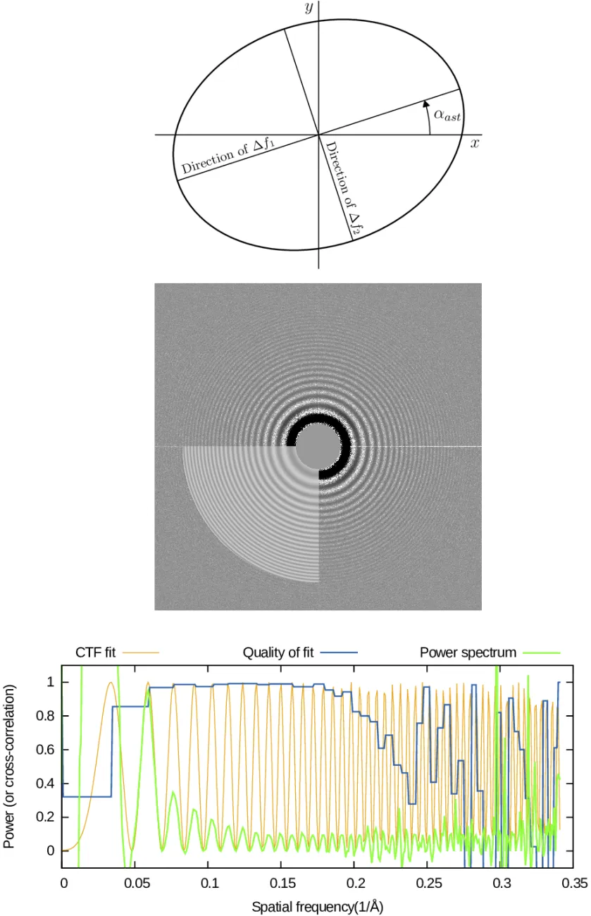
In the Find CTF panel, you can use CTFfind (Rohou & Grigorieff, 2015) to estimate CTF parameter values for each micrograph. The main parameter to be determined for each micrograph is the objective lens defocus (in Angstroms). Because in general lenses are astigmatic, one actually needs to determine two defocus values (describing defocus along the lens' major and minor axes) and the angle of astigmatism.
To estimate the values of these three defocus parameters for a micrograph, CTFfind computes a filtered version of the amplitude spectrum of the micrograph and then fits a model of the CTF (Equation 6 of Rohou & Grigorieff) to this filtered amplitude spectrum. It then returns the values of the defocus parameters which maximize the quality of the fit, as well as an image of the filtered amplitude spectrum, with the CTF model overlayed onto the lower-left quadrant. Dashed lines are also overlayed onto Fourier components where the CTF is 0.
Another diagnostic output is a 1D plot of the experimental amplitude spectrum (green), the CTF fit (orange) and the quality of fit (blue). More details on how these plots are computed is given below.
Program Options
Input Group: The group of image assets to estimate the CTF for.
Run Profile: The selected run profile will be used to run the job. The run profile describes how the job should be run (e.g. how many processors should be used, and on which different computers). Run profiles are set in the Run Profile panel, located under settings.
Expert Options
Search
Estimate Using Movies/Images: CTF Thon rings are often more visible when calculating the power spectra from the movie frames rather than the final aligned frame average. If movies are available, they should be used (this will take longer than running CTFfind on images).
No. Movie Frames to Average: When using movies, power spectra can be calculated from sub-frame averages. Thon rings are usually most visible when averaging over as many frames as are equivalent to 4 - 5 e-/Å2 (McMullan et al. 2015).
Box size (px): The dimensions of the amplitude spectrum CTFfind will compute. Smaller box sizes make the fitting process significantly faster, but sometimes at the expense of fitting accuracy. If you see warnings regarding CTF aliasing, consider increasing this parameter.
Amplitude Contrast: The fraction (between 0.0 and 1.0) of total image contrast attributed to amplitude contrast (as opposed to phase contrast), arising for example from electron scattered outside the objective aperture, or those removed by energy filtering.
Search Limits
Min. Resolution of Fit (Å): The CTF model will not be fit to regions of the amplitude spectrum corresponding to this resolution or lower.
Max. Resolution of Fit (Å): The CTF model will not be fit to regions of the amplitude spectrum corresponding to this resolution or higher.
Low Defocus For Search (Å): Positive for underfocus. The Lower bound of initial defocus search.
High Defocus For Search (Å): Positive for underfocus. Upper bound of initial defocus search.
Defocus Search Step (Å): Step size for the defocus search.
Use Slower, more Exhaustive Search? Select this if many of the movies/images are not successfully fitted.
Restrain Astigmatism? Select this if the expected astigmatism in the movies/images is small (of the order of the value entered in the next field).
Tolerated Astigmatism (Å): Astigmatism values much larger than this will be penalised. Set to negative to remove this restraint. In cases where the amplitude spectrum is very noisy, such a restraint can help achieve more accurate results.
Phase Plates
Find Additional Phase Shift? Specifies the input micrograph was recorded using a phase plate with variable phase shift, which you want to find.
Min. Phase Shift (º): If finding an additional phase shift, this value sets the lower bound for the search.
Max. Phase Shift (º): If finding an additional phase shift, this value sets the upper bound for the search.
Phase Shift Search Step (º): If finding an additional phase shift, this value sets the step size for the search.
References
Rohou A. & Grigorieff N., 2015. CTFFIND4: Fast and accurate defocus estimation from electron micrographs. J. Struct. Biol. 192, 216-221. doi:10.1016/j.jsb.2015.08.008
McMullan G., Vinothkumar K. R., Henderson R., 2015. Thon rings from amorphous ice and implications of beam-induced Brownian motion in single particle electron cryo-microscopy. Ultramicroscopy 158, 26-32. doi:10.1016/j.ultramic.2015.05.017
Picking Particles
The Find Particles Action panel allows automatic selection of particles in electron micrographs. Individual particles need to be located in each micrograph so that they may be used to compute a 3D reconstruction later. Ideally one would find all the particles and not make any erroneous selections.
In the absence of a pre-existing 3D model, one can either select (click on) each particle manually, or use the 'ab-initio' mode based on an algorithm described by Sigworth (2004). In this mode, a template is genated internally, which consists of a cosine-shaped blob and then matched against each micrographs. This works reasonably well to find globular protein complexes, even though it is less accurate and more error-prone than template-based search strategy.
Program Options
Input Group: The group of image assets in which to find particles.
Run Profile: The selected run profile will be used to run the job. The run profile describes how the job should be run (e.g. how many processors should be used, and on which different computers). Run profiles are set in the Run Profile panel, located under settings.
Maximum Particle Radius (Å): In Angstroms, the maximum radius of the particles to be found. This also determines the minimum distance between picks.
Characteristic Particle Radius (Å): In Angstroms, the radius within which most of the density is enclosed. The template for picking is a soft-edge disc, where the edge is 5 pixels wide and this parameter defines the radius at which the cosine-edge template reaches 0.5.
Threshold Peak Height: Particle coordinates will be defined as the coordinates of any peak in the search function which exceeds this threshold. In numbers of standard deviations above expected noise variations in the scoring function. See Sigworth (2004) for definition.
Avoid High Variance Areas? Avoid areas with abnormally high local variance. This can be effective in avoiding edges of support films or contamination. However, when particles generate strong contrast (e.g. in phase plate images), better results may be obtained by disabling this option.
Select Preview Image: Select an image from the Input Group to be used as a preview for the picking job. This is useful to see how different parameter settings influence the picking to tune the parameters.
Preview: Click this button to generate a preview of the picking job.
Auto Preview? Select this to generate previews automatically. Selecting different Preview Images will automatically run the picking job on the selected image and show the results.
Run Profile: The selected run profile will be used to run the job. The run profile describes how the job should be run (e.g. how many processors should be used, and on which different computers). Run profiles are set in the Run Profile panel, located under settings.
Expert Options
Highest Resolution Used in Picking (Å): The template and micrograph will be resampled (by Fourier cropping) to a pixel size of half the resolution given here. Note that the information in the 'corners' of the Fourier transforms (beyond the Nyquist frequency) remains intact, so that there is some small risk of bias beyond this resolution.
Set Minimum Distance From Edges (px): No particle shall be picked closer than this distance from the edges of the micrograph. Select to enable.
Avoid Areas With Abnormal Local Means: Avoid areas with abnormally low or high local mean. This can be effective to avoid picking from, e.g., contaminating ice crystals, support film.
Number of Background Boxes: Number of background areas to use in estimating the background spectrum. The larger the number of boxes, the more accurate the estimate should be, provided that none of the background boxes contain any particles to be picked.
Algorithm to Find Background Areas: Testing so far suggests that areas of lowest variance in experimental micrographs should be used to estimate the background spectrum. However, when using synthetic micrographs this can lead to bias in the spectrum estimation and the alternative (areas with local variances near the mean of the distribution of local variances) seems to perform better.
References
Sigworth F.J. 2004. Classical detection theory and the cryo-EM particle selection problem. J. Struct. Biol. 145, 111-122. doi:10.1016/j.jsb.2003.10.025
2D Classification
2D classification can be run using the 2D Classify Action panel. It offers a fast and robust way to assess the quality and homogeneity of a dataset. The results of classification can also be used to remove particles belonging to undesirable classes, for example classes with ill-defined features or features that suggest the presence of damaged particles or impurities.
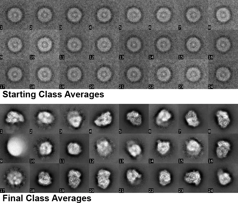
2D classification typically starts with classes calculated as averages of randomly sampled particles from the dataset. The first panel shows the first 24 out of 50 starting class averages for a dataset of VSV polymerase, a 240 kDa protein (Liang et al. 2015). The dataset was collected after the initial publication in 2015 and contained 84,608 particle images with a pixel size of 0.97 Å, cut out into 400 x 400 pixel boxes. When generating starting classes, the user has to specify the number of classes, for example 50 or 100. Furthermore, the percentage of the dataset used for the calculation has to be specified. In most cases, an average of about 200 - 300 images per class is sufficient to obtain reasonable averages (also in later refinement cycles). For example, if a dataset contains 100,000 particle images and the user requests 100 class averages, the number of particle images recommended for generating initial averages would be 100 classes x 300 images/class = 30,000 images. The percentage in this example should therefore be set to 0.3. In the case of VSV polymerase, the percentage was set to 0.18 (an average of 305 images/class). Auto Percent Used (see below) will adjust the percentage automatically.
In subsequent iteration cycles, the class averages are refined using a maximum likelihood algorithm (Sigworth 1998, Scheres et al. 2005). If the percentage is set manually, it is recommended to keep the percentage of the dataset used in the calculation unchanged for the first 10 cycles, or to increase it somewhat but remain below 100% if class averages appear very noisy. Also, the resolution limit should be set initially to 40 Å and the x,y search range should be limited in such a way that most particle displacement from the image center will be within this range. The required range will depend on the way the particles were picked. If particles are well centered after picking, the range can be set between 20 and 40 Å, otherwise a range of 100 Å or more is probably a safer option. Finally, the angular sampling rate must be set by the user. It is rarely required to choose a value below 5º and in most cases 15º is adequate. All four options (percentage, resolution limit, search range, angular sampling rate) can significantly speed up computation and it is therefore worth setting these carefully. For the VSV polymerase dataset, the class averages shown in the second panel were obtained after 20 cycles with automatically adjusted resolution, including 5 cycles at 7 Å resolution and using the full dataset, a search range of 40 Å and a sampling rate of 15º. Many of the class averages show clear secondary structure (α-helixes).
Program Options
Input Refinement Package: The name of the refinement package previously set up in the Assets panel (providing details of particle locations, box size and imaging parameters).
Input Starting References: A set of class averages from a previous run of 2D classification. If no prior class averages are available, the option New Classification can be selected, allowing the user to enter the number of desired classes in the next menu.
No. of Classes: The number of classes that should be generated. This input is only available when starting a fresh classification run.
No. of Cycles to Run: The number of refinement cycles to run. If the option Auto Percent Used is selected, 20 cycles are usually sufficient to generate good class averages. If the user decides to set parameters manually, 5 to 10 cycles are usually sufficient for a particular set of parameters. Several of these shorter runs should be used to obtain final class averages, updating parameters as needed (e.g. Percent Used, see example above).
Expert Options
Low-Resolution Limit (Å): The data used for classification is usually bandpass-limited to exclude spurious low-resolution features in the particle background (set by the low-resolution limit) and high-resolution noise (set by the high-resolution limit, see next two input fields). It is good practice to set the low-resolution limit to 2.5x the approximate particle mask radius.
Low-Resolution Limit (Start/Finish) (Å): The high-resolution limit should be selected to remove data with low signal-to-noise ratio, and to help speed up the calculation. For example, setting the final high-resolution limit to 8 Å includes signal originating from protein secondary structure that often helps generate recognizable features in the class averages (see example above). The starting limit should be set to a lower resolution, for example 20 to 40 Å, to help convergence of the algorithm. The limit will be incremented in each cycle to the final specified resolution.
Mask Radius (Å): The radius of the circular mask applied to the input class averages before classification starts. This mask should be sufficiently large to include the largest dimension of the particle. The mask helps remove noise outside the area of the particle.
Angular Search Step (º): The angular step used to generate the search grid when marginalizing over the in-plane rotational alignment parameter. The smaller the value, the finer the search grid and the slower the search. It is often sufficient to set the step to 15º as the algorithm varies the starting point of the grid in each refinement cycle, thereby covering intermediate in-plane alignment angles. However, users can try to reduce the step to 5º (smaller is probably not helpful) to see if class averages can be improved further once no further improvement is seen at 15º.
Search Range in X/Y (Å): The search can be limited in the X and Y directions (measured from the box center) to ensure that only particles close to the box center are used for classification. A smaller range, for example 20 to 40 Å, can speed up computation. However, the range should be chosen sufficiently generously to capture most particles. If the range of particle displacements from the box center is unknown, start with a larger value, e.g. 100 Å, check the results when the run finishes and reduce the range appropriately.
Smoothing Factor: A factor that reduces the range of likelihoods used during classification. A reduced range can help prevent the appearance of "empty" classes (no members) early in the classification. Soothing may also suppress some high-resolution noise. The user should try values between 0.1 and 1 if classification suffers from the disappearance of small classes or noisy class averages.
Exclude Blank Edges? Should particle boxes with blank edges be excluded from classification? Blank edges can be the result of particles selected close to the edges of micrographs. Blank edges can lead to errors in the calculation of the likelihood function, which depends on the noise statistics.
Auto Percent Used? Should the percent of included particles be adjusted automatically? A classification scheme using initially 300 particles/class, then 30% and then 100% is often sufficient to obtain good classes and this scheme will be used when this option is selected.
Percent Used: The fraction of the dataset used for classification. Especially in the beginning, classification proceeds more rapidly when only a small number of particles are used per class, e.g. 300 (see example above). Later runs that refine the class averages should use a higher percentage and the final run(s) should use all the data. This option is only available when Auto Percent Used is not selected.
References
Sigworth, F. J., 1998. A maximum-likelihood approach to single-particle image refinement. J. Struct. Biol. 122, 328-339. dio:10.1006/jsbi.1998.4014
Scheres, S. H. W., Valle, M., Nuñez, R., Sorzano, C. O. S., Marabini, R., Herman, G. T. & Jose-Maria Carazo, J.-M., 2005. Maximum-likelihood multi-reference refinement for electron microscopy images. J. Mol. Biol. 348, 139-149. doi:10.1016/j.jmb.2005.02.031
Liang, B., Li, Z., Jenni, S., Rahmeh, A. A., Morin, B. M., Grant, T., Grigorieff, N., Harrison, S. C. & Whelan, S. P., 2015. Structure of the L protein of vesicular stomatitis virus from electron cryomicroscopy. Cell 162, 314-327. doi:10.1016/j.cell.2015.06.018
Ab-Initio 3D Reconstruction
Ab-initio 3D Volumes can be generated using the Ab Initio 3D Actions panel. When a prior 3D reconstruction of a molecule or complex is available that has a closely related structure, it is usually fastest and safest to use it to initialize 3D refinement and reconstruction of a new dataset. However, in many cases such a structure is not available, or an independently determined structure is desired. Ab-initio 3D reconstruction offers a way to start refinement and reconstruction without any prior structural information. The figure shows an ab-initio 3D reconstruction of VSV polymerase (Liang et al. 2015):
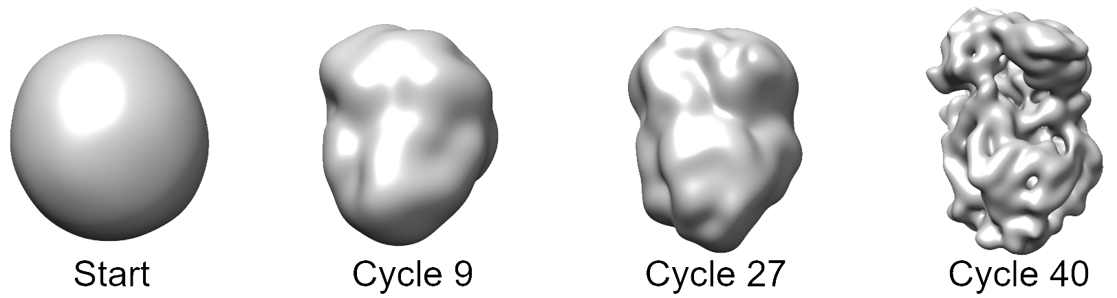
It is advisable to precede the ab-initio step with a 2D classification step to remove junk particles and select a high-quality subset of the data. Furthermore, it may be helpful to select particles from images that are defocused by 1.5 µm or more. A refinement package has to be created (in Assets) that will be used with the ab-initio procedure, either from selected 2D classes or using picked particle position. The idea of the ab-initio algorithm is to iteratively improve a 3D reconstruction, starting with a reconstruction calculated from random Euler angles, by aligning a small percentage of the data against the current reconstruction and increasing the refinement resolution and percentage at each iteration (Grigorieff, 2016). This procedure can also be carried out using multiple references that must be specified when creating the refinement package. The procedure stops after a user-specified number of refinement cycles and restarts if more than one starts are specified.
The progress of the ab-initio reconstruction is displayed as a plot of the average sigma value that measures the average apparent noise-to-signal ratio in the data. The sigma value should decrease as the reconstruction gets closer to the true structure. The current reconstruction is also displayed as three orthogonal central slices and three orthogonal projections.
If the ab-initio procedure fails on a symmetrical particle, users should repeat it using C1 (no symmetry). This can be specified by creating a new refinement package that is based on the previous refinement package, and changing the symmetry to C1. If a particle is close to spherical, such as apoferritin, it may be necessary to change the initial and final resolution limits from 40 Å and 9 Å (default) to higher resolution, e.g. 15 Å and 6 Å (see Expert Options). Finally, it is worth repeating the procedure a few times if a good reconstruction is not obtained in the first trial.
Program Options
Input Refinement Package: The name of the refinement package previously set up in the Assets panel (providing details of particle locations, box size and imaging parameters).
Number of Starts: The number of times the ab-initio reconstruction is restarted, using the result from the previous run in each restart.
No. of Cycles per Start: The number of refinement cycles to run for each start. The percentage of particles and the refinement resolution limit will be adjusted automatically from cycle to cycle using initial and final values specified under Expert Options.
Expert Options
Initial Resolution Limit (Å): The starting resolution limit used to align particles against the current 3D reconstruction. In most cases, this should specify a relatively low resolution to make sure the reconstructions generated in the initial refinement cycles do not develop spurious high-resolution features.
Final Resolution Limit (Å): The resolution limit used in the final refinement cycle. In most cases, this should specify a resolution at which expected secondary structure becomes apparent, i.e. around 9 Å.
Use Auto-Masking? Should the 3D reconstructions be masked? Masking is important to suppress weak density features that usually appear in the early stages of ab-initio reconstruction, thus preventing them to get amplified during the iterative refinement. Masking should only be disabled if it appears to interfere with the reconstruction process.
Auto Percent used? Should the percentage of particles used in each refinement cycle be set automatically? If reconstructions appear very noisy or reconstructions settle into a wrong structure that does not change anymore during iterations, disable this option and specify initial and final percentages manually. To reduce noise, increase the percentage; to make reconstructions more variable, decrease the percentage. By default, the initial percentage is set to include an equivalent of 2500 asymmetric units and the final percentage corresponds to 10,000 asymmetric units used.
Initial % Used / Final % Used: User-specified percentages of particles used when Auto Percent Used is disabled.
Apply Likelihood Blurring? Should the reconstructions be blurred by inserting each particle image at multiple orientations, weighted by a likelihood function? Enable this option if the ab-initio procedure appears to suffer from over-fitting and the appearance of spurious high-resolution features.
Smoothing Factor: A factor that reduces the range of likelihoods used for blurring. A smaller number leads to more blurring. The user should try values between 0.1 and 1.
References
Grigorieff, N., 2016. Frealign: An exploratory tool for single-particle cryo-EM. Methods Enzymol. 579, 191-226. doi:10.1016/bs.mie.2016.04.013
Liang, B., Li, Z., Jenni, S., Rahmeh, A. A., Morin, B. M., Grant, T., Grigorieff, N., Harrison, S. C., Whelan, S. P., 2015. Structure of the L protein of vesicular stomatitis virus from electron cryomicroscopy. Cell 162, 314-327. doi:10.1016/j.cell.2015.06.018
Automatic Refinement
This Auto Refine Actions panel allows users to refine a 3D reconstruction to high resolution using Frealign (Grigorieff, 2016) without the need to set many of the parameters that are required for manual refinement (see Manual Refine panel). In the simplest case, all that is required is the specification of a refinement package (set up under Assets), a starting reference (for example, a reconstruction obtained from the ab-initio procedure) and an initial resolution limit used in the refinement. The resolution should start low, for example at 30 or 40 Å, to remove potential bias in the starting reference. However, for particles that are close to spherical, such as apoferritin, a higher resolution should be specified, between 8 and 12 Å (see Expert Options).
Program Options
Starting Reference: The initial 3D reconstruction used to align particles against. This should be of reasonable quality to ensure successful refinement.
Initial Res. Limit (Å): The starting resolution limit used to align particles against the starting reference. In most cases, this should specify a relatively low resolution to remove potential bias in the starting reference.
Refinement Run Profile: The run profile used for particle alignment. This can be set to a large number if desired and CPUs are available, for example 300 or 1000. The alignment job will be divided into smaller jobs accordingly. The user is encouraged to test which number to use to achieve the best compromise between job time and resource requirements.
Reconstruction Run Profile: The run profile used for calculating 3D reconstructions. The reconstruction will be divided into multiple reconstructions, each using part of the data. A merge step at the end is then executed to calculate the final reconstruction. It is advisable not to use more than 50 - 100 CPUs for reconstructions to limit the number of intermediate reconstruction dump files. Writing and reading more than 100 will limit the speed of the job due to disk speed limitations and may also require large amounts of free disk space.
Expert Options
General Refinement
Low/High-Resolution Limit (Å): The data used for refinement is usually bandpass-limited to exclude spurious low-resolution features in the particle background (set by the low-resolution limit) and high-resolution noise (set by the high-resolution limit). It is good practice to set the low-resolution limit to 2.5x the approximate particle mask radius. The high-resolution limit should remain significantly below the resolution of the reference used for refinement to enable unbiased resolution estimation using the Fourier Shell Correlation curve.
Inner/Outer Mask Radius (Å): Radii describing a spherical mask with an inner and outer radius that will be applied to the final reconstruction and to the half reconstructions to calculate Fourier Shell Correlation curve. The inner radius is normally set to 0.0 but can assume non-zero values to remove density inside a particle if it represents largely disordered features, such as the genomic RNA or DNA of a virus.
Global Search
Global Mask Radius (Å): The radius describing the area within the boxed-out particles that contains the particles. This radius us usually larger than the particle radius to account for particles that are not perfectly centered. The best value will depend on the way the particles were picked.
Number of Results to Refine: For a global search, an angular grid search is performed and the alignment parameters for the N best matching projections are then refined further in a local refinement. Only the set of parameters yielding the best score (correlation coefficient) is kept. Increasing N will increase the chances of finding the correct particle orientations but will slow down the search. A value of 20 is recommended.
Search Range in X/Y (Å): The global search can be limited in the X and Y directions (measured from the box center) to ensure that only particles close to the box center are found. This is useful when the particle density is high and particles end up close to each other. In this case, it is usually still possible to align all particles in a cluster of particles (assuming they do not significantly overlap). The values provided here for the search range should be set to exclude the possibility that the same particle is selected twice and counted as two different particles.
Reconstruction
Autocrop Images? Should the particle images be cropped to a minimum size determined by the mask radius to accelerate 3D reconstruction? This is usually not recommended as it increases interpolation artifacts.
Apply Likelihood Blurring? Should the reconstructions be blurred by inserting each particle image at multiple orientations, weighted by a likelihood function? Enable this option if the ab-initio procedure appears to suffer from over-fitting and the appearance of spurious high-resolution features.
Smoothing Factor: A factor that reduces the range of likelihoods used for blurring. A smaller number leads to more blurring. The user should try values between 0.1 and 1.
Masking
Use Auto-Masking? Should the 3D reconstructions be masked? Masking can suppress spurious density features that could be amplified during the iterative refinement. Masking should only be disabled if it appears to interfere with the reconstruction process.
References
Grigorieff, N., 2016. Frealign: An exploratory tool for single-particle cryo-EM. Methods Enzymol. 579, 191-226. doi:10.1016/bs.mie.2016.04.013
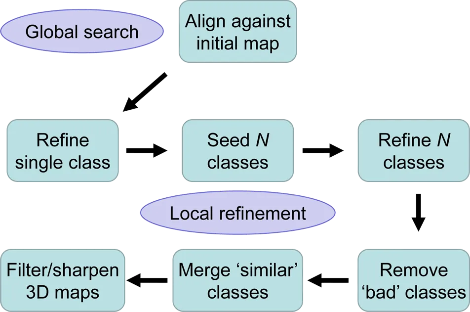
Manual Refinement
The goal of refinement and reconstruction is to obtain 3D maps of the imaged particle at the highest possible resolution. Refinement typically starts with a preexisting structure that serves as a reference to determine initial particle alignment parameters using a global parameter search. In subsequent iterations, these parameters are refined and (optionally) the dataset can be classified into several classes with distinct structural features.
The Manual Refine Action panel allows the user to define a refinement job that includes a set number of iterations (refinement cycles) and number of desired classes to be generated (Lyumkis et al. 2013). The general refinement strategies and options are similar to those available with Frealign and are described in Grigorieff, 2016.
In each refinement cycle, the particle parameters are aligned in a local search (searching only parameters close to those found in the previous cycle) against the reconstruction (or reconstructions if more than one class is refined) obtained in the previous cycle. The final result includes refined alignment parameters, class memberships (occupancies) and filtered 3D reconstructions (Sindelar and Grigorieff, 2012) for all classes. Further refinement can be performed with different numbers of classes by setting up a new refinement package and selecting reconstructions and particles of classes from a previous package as input for the new package. To bring out high-resolution features in the maps, the user should sharpen the reconstructions by applying a negative B-factor, for example using the external program bfactor or using the Finalize Actions panel. The diagram shows a typical workflow.
Program Options
Input Refinement Package: The name of the refinement package previously set up in the Assets panel (providing details of particle locations, box size and imaging parameters).
Input Parameters: The source of the starting parameters for this refinement run. These can be either set to be random Euler angles and zero X,Y shifts, or they can be the output of a previous refinement (if available).
Use a Mask? Should the input 3D reference be masked using a 3D mask? The 3D mask has to be defined by a separate 3D Volume asset. Density values larger than 0 will be considered inside the mask, 0 and below will be considered outside the mask. Additional masking parameters are defined in the Masking section below.
Local Refinement/Global Search: If no starting parameters from a previous refinement are available, they have to be determined in a global search (slow); otherwise it is usually sufficient to perform local refinement (fast).
No. of Cycles to Run: The number of refinement cycles to run. For a global search, one is usually sufficient, possibly followed by another one at a later stage in the refinement if the user suspects that the initial reference was limited in quality such that a significant number of particles were misaligned. For local refinement of a single class, typically 3 to 5 cycles are sufficient, possibly followed by another local refinement at increased resolution (see below). If multiple classes are refined, between 30 and 50 cycles should be run to ensure convergence of the classes.
Hi-Res Limit (Å): The data used for refinement is usually bandpass-limited to exclude spurious low-resolution features in the particle background (determined by the low-resolution limit, see Expert Options) and high-resolution noise (determined by the high-resolution limit set here). The high-resolution limit should remain significantly below the resolution of the reference used for refinement to enable unbiased resolution estimation using the Fourier Shell Correlation curve.
Refinement Run Profile: The run profile used for particle alignment. This can be set to a large number if desired and CPUs are available, for example 300 or 1000. The alignment job will be divided into smaller jobs accordingly. The user is encouraged to test which number to use to achieve the best compromise between job time and resource requirements.
Reconstruction Run Profile: The run profile used for calculating 3D reconstructions. The reconstruction will be divided into multiple reconstructions, each using part of the data. A merge step at the end is then executed to calculate the final reconstruction. It is advisable not to use more than 50 - 100 CPUs for reconstructions to limit the number of intermediate reconstruction dump files. Writing and reading more than 100 will limit the speed of the job due to disk speed limitations and may also require large amounts of free disk space.
Expert Options
Parameters to Refine
Psi, Theta, Phi, X Shift, Y Shift: Check all the parameters that should be refined. Psi is the in-plane angle; Theta is the out-of-plane angle.
General Refinement
Low-Resolution Limit (Å): The low-resolution limit used to band-pass filter the input particle images. It is good practice to set the low-resolution limit to 2.5x the approximate particle mask radius.
Outer Mask Radius (Å): The radius of the circular mask applied to the input images before refinement starts. This mask should be sufficiently large to include the largest dimension of the particle. When a global search is performed, the radius should be set to include the expected area containing the particle. This area is usually larger than the area defined by the largest dimension of the particle because particles may not be precisely centered.
Inner Mask Radius (Å): The radius of the circular mask applied to the input 3D reference. The inner radius is normally set to 0.0 but can assume non-zero values to remove density inside a particle if it represents largely disordered features, such as the genomic RNA or DNA of a virus.
Signed CC Resolution Limit (Å): Particle alignment is done by maximizing a correlation coefficient with the reference. The user has the option to maximize the unsigned correlation coefficient instead (starting at the limit set here) to reduce overfitting (Stewart and Grigorieff, 2004). Overfitting is also reduced by appropriate weighting of the data and this is usually sufficient to achieve good refinement results. The limit set here should therefore be set to 0.0 to maximize the signed correlation at all resolutions, unless there is evidence that there is overfitting. (This feature was formerly known as "FBOOST".)
Percent Used (%): The fraction of the data used for refinement and reconstruction. Using less than 100%, for example 10 or 20%, may increase the convergence radius of the refinement. A refinement should always be finished with a few cycles using 100% of the data.
Global Search
Global Mask Radius (Å): The radius of the circular mask applied to the input images before the global search starts. This can be the same as the Outer Mask Radius (see above) but could also be chosen larger if particles are not well centered inside the box.
Number of Results to Refine: For a global search, an angular grid search is performed and the alignment parameters for the N best matching projections are then refined further in a local refinement. Only the set of parameters yielding the best score (correlation coefficient) is kept. Increasing N will increase the chances of finding the correct particle orientations but will slow down the search. A value of 20 is recommended.
Also Refine Input Parameters? In addition to the N best sets of parameter values found during the grid search, the input set of parameters is also locally refined. Switching this off can help reduce over-fitting that may have biased the input parameters.
Angular Search Step (°): The angular step used to generate the search grid for the global search. An appropriate value is suggested by default (depending on particle size and high-resolution limit) but smaller values can be tried if the user suspects that the search misses orientations found in the particle dataset. The smaller the value, the finer the search grid and the slower the search.
Search Range in X/Y (Å): The global search can be limited in the X and Y directions (measured from the box center) to ensure that only particles close to the box center are found. This is useful when the particle density is high and particles end up close to each other. In this case, it is usually still possible to align all particles in a cluster of particles (assuming they do not significantly overlap). The values provided here for the search range should be set to exclude the possibility that the same particle is selected twice and counted as two different particles.
Classification
High-Resolution Limit (Å): The limit set here is analogous to the high-resolution limit set for refinement. It cannot exceed the refinement limit. Setting it to a lower resolution may increase the useful SNR for classification and lead to better separation of particles with different structural features. However, at lower resolution the classification may also become less sensitive to heterogeneity represented by smaller structural features.
Focused Classification? Classification can be performed based on structural variability in a defined region of the particle. This is useful when there are multiple regions that have uncorrelated structural variability. Using focused classification, each of these regions can be classified in turn. The focus feature can also be used to reduce noise from other parts of the images and increase the useful SNR for classification. The focus region is defined by a sphere with coordinates and radius in the following four inputs. (This feature was formerly known as "focus_mask".)
Sphere X/Y/Z Co-ordinate and Radius (Å): These values describe a spherical region inside the particle that contains the structural variability to focus on.
CTF
CTF Refinement
Refine CTF? Should the CTF be refined as well? This is only recommended for high-resolution data that yield reconstructions of better than 4 Å resolution, and for particles of sufficient molecular mass (500 kDa and higher).
Defocus Search Range (Å): The range of defocus values to search over for each particle. A search with the step size given in the next input will be performed starting at the defocus values determined in the previous refinement cycle minus the search range, up to values plus the search range. The search steps will be applied to both defocus values, keeping the estimated astigmatism constant.
Defocus Search Step (Å): The search step for the defocus search.
Reconstruction
Score to Weight Constant (Å2): The particles inserted into a reconstruction will be weighted according to their scores. The weighting function is akin to a B-factor, attenuating high-resolution signal of particles with lower scores more strongly than of particles with higher scores. The B-factor applied to each particle prior to insertion into the reconstruction is calculated as B = (score - average score) * constant * 0.25. Users are encouraged to calculate reconstructions with different values to find a value that produces the highest resolution. Values between 0 and 10 are reasonable (0 will disable weighting).
Adjust Score for Defocus? Scores sometimes depend on the amount of image defocus. A larger defocus amplifies low-resolution features in the image and this may lead to higher particle scores compared to particles from an image with a small defocus. Adjusting the scores for this difference makes sure that particles with smaller defocus are not systematically downweighted by the above B-factor weighting.
Score Threshold: Particles with a score lower than the threshold will be excluded from the reconstruction. This provides a way to exclude particles that may score low because of misalignment or damage.
Resolution Limit (Å): The reconstruction calculation can be accelerated by limiting its resolution. It is important to make sure that the resolution limit entered here is higher than the resolution used for refinement in the following cycle.
Autocrop Images? The reconstruction calculation can also be accelerated by cropping the boxes containing the particles. Cropping will slightly reduce the overall quality of the reconstruction due to increased aliasing effects and should not be used when finalizing refinement. However, during refinement, cropping can greatly increase the speed of reconstruction without noticeable impact on the refinement results.
Apply Likelihood Blurring? Should the in-plane orientation and X/y shifts be blurred by a likelihood function to increase the convergence radius of the refinement?
Smoothing Factor: If likelihood blurring is applied, this factor reduces the range of likelihoods used blurring. The user should try values between 0.1 (more blurring) and 1 (less blurring).
Masking
Use Auto Masking? Should the 3D reconstruction be automatically masked between refinement cycles to suppress noise?
Mask Edge Width (Å): If a 3D Volume is used for masking (see above), a soft edge with a width specified here will be added.
Outside Weight: By default, densities outside the mask will be set to the average of the density outside (this is akin to solvent flattening). However, in some cases, it is better to maintain a low-pass filtered version of the outside. For example, the alignment of membrane proteins can be improved if the inside of the 3D mask outlines the protein and a low-pass filtered version of the outside density is included to reflect the density of the detergent micelle.
Low-Pass Filter Outside Mask? Should the density outside the mask be low-pass filtered (if the Outside Weight is not zero)? This may be useful in the alignment of membrane proteins that have a disordered detergent micelle (see previous parameter).
Filter Resolution (Å): The resolution of the low-pass filter to be applied.
References
Stewart, A., Grigorieff, N., 2004. Noise bias in the refinement of structures derived from single particles. Ultramicroscopy 102, 67-84. dio:10.1016/j.ultramic.2004.08.008
Sindelar, C. V., Grigorieff, N., 2012. Optimal noise reduction in 3D reconstructions of single particles using a volume-normalized filter. J. Struct. Biol. 180, 26-38. dio:10.1016/j.jsb.2012.05.005
Lyumkis, D., Brilot, A. F., Theobald, D. L., Grigorieff, N., 2013. Likelihood-based classification of cryo-EM images using FREALIGN. J. Struct. Biol. 183, 377-388. dio:10.1016/j.jsb.2013.07.005
Grigorieff, N., 2016. Frealign: An exploratory tool for single-particle cryo-EM. Methods Enzymol. 579, 191-226. doi:10.1016/bs.mie.2016.04.013
3D Classification
For 3D classification, it is recommended in most cases to first refine with a single class (see "How do I start 3D classification?" in FAQs). This saves time since only one class is refined, and it ensures that the classes that emerge out of classification will be all be roughly aligned with each other, making it easier to recognize structural differences between the classes. However, if particles in a dataset vary significantly in size and structure, it may be better to refine with several classes from the beginning, skipping the refinement with a single class.
3D classification starts with the creation of a Refinement Package that specifies the number of desired classes. Follow the steps described in Refinement Package Assets and create a Refinement Package either using another Refinement Package as a template, or by creating one based on Particle Positions or 2D class averages. The number of 3D classes has to be specified in the field “Number of classes for 3D refinement” when running the Refinement Package wizard.
When using a Refinement Package as a template that has more than one class (from an earlier 3D classification), the wizard solicits a number of additional questions that allows the user to select which of the existing classes (particles and alignment parameters) will be used, and how to assign these classes to the classes in the new Refinement Package. A particle is assigned to the class for which it has the highest occupancy. Classes can be excluded from the new Refinement Package by answering No to “Carry over all particles?” The corresponding particles will be excluded from the newly created stack and subsequent refinement. All classes that are carried forward can then be assigned to the classes in the new Refinement Package. This step also allows the combination of several classes into a single new class. Therefore, using the wizard, all possible combinations of class selections and removals are possible.
To start refinement and classification with the new Refinement Package, use the Auto Refine or Manual Refine Action and select the new Refinement Package as the active input for the refinement. Active references for each of the classes in a Refinement Package can be selected or changed in the Assets panel, as well as in the Manual Refine Actions panel. When running Auto Refine, the starting references will always be generated from the parameters after randomizing the particle occupancies.
Map Sharpening
The high-resolution signal in 3D reconstructions is usually dampened by various factors, including the envelope function affecting the CTF of the microscope, the modulation transfer function (MTF) of the detector, beam-induced motion, and alignment and interpolation errors introduced during image processing. Structural heterogeneity present in the particles may also contribute. It is common practice to express this dampening by a B-factor, expressed in Å2 and given as exp(-0.25 B/d2) where d is the resolution (in Å) at which the dampening occurs. To visualize the high-resolution details in a reconstructed map, its amplitudes have to be restored by applying a negative B-factor, thereby sharpening the map. The following figure shows an example of 3-Å map of VSV polymerase (Liang et al. 2015) before and after sharpening:
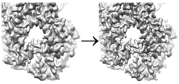
This panel provides the user with a few parameters to sharpen a map. In the simplest case, a map can be sharpened by providing a negative B-factor. However, because B-factor sharpening involves multiplication with an exponential function, the noise at high resolution can easily be over-amplified. A more robust method to restore the amplitudes at high resolution that also works if the dampening cannot be described with a simple B-factor can be achieved by flattening (i.e. whitening) the amplitude spectrum at high resolution. The panel provides a flexible way to combine B-factor sharpening and spectral flattening to optimize the visibility of high-resolution details in the final map. Optionally, the resolution statistics can be used to apply figure-of-merit (FOM) weighting (Rosenthal & Henderson, 2003) and a 3D mask can be supplied to remove background noise from the map for more accurate sharpening. Finally, the handedness of the map can be inverted if it is wrong and the real-space dampening of densities near the edge of the reconstruction box due to trilinear interpolation used during reconstruction can be corrected.
Program Options
Input Volume: The volume (reconstruction) to be sharpened.
Supply a Mask? Should the volume be masked to make sharpening more accurate? If checked, a volume containing the 3D mask must be selected.
Flatten From Res. (Å): The low-resolution limit of the part of the amplitude spectrum to be flattened (whitened). This should normally be a resolution beyond which the influence of the shape transform of the particle is negligible, between 8 – 10 Å.
Resolution Cut-Off (Å): The high-resolution limit applied to the sharpened map. The filter edge is given by a cosine function of width specified by “Filter Edge-Width.”
Pre-Cut-Off B-Factor (Å2): The B-factor to be applied to the low-resolution end of the amplitude spectrum, up to the point given as “Flatten From Res.” A B-factor of -90 Å2 is usually appropriate for cryo-EM maps calculated using data collected on direct detectors.
Post-Cut-Off B-Factor (Å2): The B-factor to be applied to the high-resolution end of the amplitude spectrum, from to the point given as “Flatten From Res.” This will apply a B-factor after flattening the spectrum. A value between 0 and 25 Å2 is usually appropriate since the flattening should restore most of the high-resolution signal without the need for further amplification.
Filter Edge-Width (Å): The width of the cosine edge of the resolution cut-off applied to the final sharpened map. The width of the cosine is given as 1/w, where w is the value entered here.
Use FOM Weighting? Should the sharpened map be weighted using a figure of merit (FOM) derived from the resolution statistics describing the map (see Rosenthal & Henderson, 2003)?
SSNR Scale Factor: The FOM values are calculated as SSNR/(1+SSNR) where SSNR is the spectral signal-to-noise ratio of the map to be sharpened (calculated as part of the reconstruction). The scale factor allows users to change the effective SSNR values used in this calculation. This can be useful, for example, if the SSNR represents the average signal in a reconstruction but FOM weighting should be performed using a higher SSNR that represents the signal when more disordered parts are excluded from the map. A higher SSNR leads to less filtering that may be more appropriate for high-resolution details in the better parts of a map.
Inner Mask Radius (Å): The radius describing the inner bounds of the particle. This is usually set to 0 unless the particle is hollow or has largely disordered density in its center, such as the genome of a spherical virus.
Outer Mask Radius (Å): The radius describing the outer bounds of the particle. A spherical mask with this radius will be applied to the map before sharpening unless a 3D mask volume is supplied.
Invert Handedness? Should the handedness of the sharpened map be inverted? If a reconstruction was initiated using the ab-initio procedure, the handedness will be undetermined and may have to be inverted if found incorrect.
Correct Gridding Error: Should the real-space dampening of the densities near the edge of the reconstruction box be corrected? The dampening is described by a sinc function and results from the trilinear interpolation used during 3D reconstruction.
References
Liang, B., Li, Z., Jenni, S., Rahmeh, A. A., Morin, B. M., Grant, T., Grigorieff, N., Harrison, S. C., Whelan, S. P., 2015. Structure of the L protein of vesicular stomatitis virus from electron cryomicroscopy. Cell 162, 314-327. doi:10.1016/j.cell.2015.06.018
Rosenthal, P. B. & Henderson, R., 2003. Optimal determination of particle orientation, absolute hand, and contrast loss in single-particle electron cryomicroscopy. J. Mol. Biol. 333, 721-745. doi.org/10.1016/j.jmb.2003.07.013
Settings
cisTEM can be run on a local workstation or remotely on a computer cluster. After installation, appropriate Run Profiles should be defined under Settings. The Settings panel can be used to manage Run Profiles that specify where cisTEM runs its jobs and how many jobs are run in parallel to speed up processing. cisTEM runs jobs through a job manager. A set of default profiles can be stored in a file called default_run_profiles.txt and placed into the bin directory containing the cisTEM executable. On startup, cisTEM loads the file and makes the Run Profiles available to all users. It is recommended to set up such defaults when cisTEM is installed to enable users to easily run jobs. cisTEM comes with a Run Profile to run on a local workstation with 20 CPU cores.
A Run Profile specifies the path for the manager command, as well as for the different job commands used to perform Actions (for example, Unblur, CTFfind). In the simplest case, all of these commands are located in the cisTEM bin directory and the bin directory is contained in the PATH environment variable. This will make the commands accessible by executing the name of the command without an additional path or directory. If the bin directory is not contained in the PATH environment variable, the full directory path has to be given (see below).
Run Profiles can be created, edited and deleted, imported from a file and exported to a file, for example default_run_profiles.txt. To create a new Run Profile, click Add next to the list of profiles on the left, then select the new profile from the list. Double-click on the name to rename it as desired. To create a profile that executes jobs locally, click on Add under the large Command box. This adds a line with the text $command and specifying a single copy with a 100 ms delay time. Double-click on the newly created line and edit the number of copies to run. When run locally, this should be the number of CPU cores available on the machine, plus 1 for the manager command. For example, if a workstation has 16 CPU cores, the number of copies to run should be set to 17 to make full use of the workstation. Click OK to accept the updated number of copies, then click Save to save the changes to the Run Profile. The Launch Delay does not usually have to be adjusted.
If the path to the cisTEM bin directory must be included (see above), add the full path to the manager command (the line with $command), double-click on the line in the large Command box and add the path again to the line containing $command. Click OK, then Save to save the changes.
The following lines provide examples of Run Profiles for more complicated computational infrastructure. Add the appropriate profiles to default_run_profiles.txt to make them available to all users. The examples assume that cisTEM is run on a workstation that has ssh access to the cluster head node. If this type of access is not available, it is recommended to run an interactive session on one of the cluster nodes. When the cisTEM GUI is run on a cluster node, the manager command line comes simply $command or /cisTEM_bin_directory/$command.
SGE cluster
Manager command
ssh -f head_node 'nohup /cisTEM_bin_directory/$command'
Job command
qsub -N cisTEM -j y -o /dev/null -b y -cwd -V /cisTEM_bin_directory/$command
LSF cluster
Manager command
ssh -f head_node 'nohup /cisTEM_bin_directory/$command'
Job command
bsub -J cisTEM -n 1 -o /dev/null /cisTEM_bin_directory/$command
SLURM cluster with srun
Manager command
ssh -f head_node 'nohup /cisTEM_bin_directory/$command'
Job command
srun -n 1 -o /dev/null /cisTEM_bin_directory/$command
SLURM cluster with sbatch
Manager command
ssh -f head_node 'nohup /cisTEM_bin_directory/$command'
Job command
sbatch --export=c='$command' /cisTEM_bin_directory/slurm.sh
The slurm.csh script must be made executable (chmod +x slurm.csh) and contain the following lines:
#!/bin/bash
#SBATCH --nodes 1
#SBATCH --ntasks-per-node=1
#SBATCH --mem-per-cpu 5000
#SBATCH --time 120:00:00
#SBATCH --partition general
#SBATCH --mail-type=ALL
#SBATCH -o slurm.%j.out
#SBATCH -e slurm.%j.err
$c
SSH cluster
An "SSH cluster" is not a real cluster; it consists of independent workstations that are SSH-accessible and share diskspace. Using the following Run Profile, a job can be distributed over several workstations. The number of jobs to run on each workstation can be set for each job command line.
Manager command
ssh -f head_node 'nohup /cisTEM_bin_directory/$command'
Job command to include three workstations named machine1, machine2 and machine3
ssh -f machine1 /cisTEM_bin_directory/$command
ssh -f machine2 /cisTEM_bin_directory/$command
ssh -f machine3 /cisTEM_bin_directory/$command
Torque cluster
Please read Reply #7 of Forum topic "Unable to get a cisTEM job to parallelize on multiple nodes in cluster" for further details.
Database Commands
cisTEM stores all the meta data information in an SQLite database. This makes it possible to interact with the database using the sqlite3 command line program, and SQL commands. To open a database with sqlite3, simply run
sqlite3 my_database.db
Once connected, typing
.tables
(include the "."), will list all tables that the data is stored in, typing
.schema name_of_table
will give you information about what is in that particular table. It is fairly straightforward to manipulate the database with some experience with SQL. It is also possible to run an SQL query in a single line. This is useful for quick queries, or for incorporating the query into a script. In this case, simply run
sqlite3 my_database.db "desired command"
By default the output from a query will be returned using “|” as the separator between columns. This default behavior can be changed by providing the -separator argument, e.g. to run a query where the output is separated by spaces run
sqlite3 -separator ' ' database_name.db "desired command"
To quit sqlite3, type
.quit
Below are a number of examples for retrieving specific information from the database.
Images in a Group
The filenames and x,y positions of all particle position assets in a specific image group can be retrieved using the following procedure:
1) Determine the group ID for the desired group. Within sqlite3, run
select * from image_group_list;
(include the ";" at the end). This will produce a list of the image groups with their IDs in the first column.
2) Run the command below, replacing $group_id (it appears twice) with the ID of the desired group to obtain the filenames of all the members in the group:
select filename from image_assets, image_group_$group_id where image_assets.image_asset_id = image_group_$group_id.image_asset_id;
e.g. to obtain the filenames of all the images in group 1, type
select filename from image_assets, image_group_1 where image_assets.image_asset_id = image_group_1.image_asset_id;
Particle Positions
The filenames and x,y positions of all particle position assets can be retrieved by running (within sqlite3):
select filename, x_position, y_position from image_assets, particle_position_assets where image_assets.image_asset_id = particle_position_assets.parent_image_asset_id;
It is also possible to access only the particle position information for the particles in a given refinement package, or to compare particles between refinement packages. Determine the ID for the desired refinement package by running
select * from refinement_package_assets;
This will return a list of all refinement packages with their IDs in the first column. To return a list of all the original position asset IDs for a given refinement_package_id, use
select original_particle_position_asset_id from refinement_package_contained_particles_$wanted_id;
For example, to return all the positions for the refinement package with the ID 1, use
select original_particle_position_asset_id from refinement_package_contained_particles_1;
If there are two refinement packages, created from the same initial refinement package, the particles contained in both packages can be listed using
select refinement_package_contained_particles_$first_id.original_particle_position_asset_id from refinement_package_contained_particles_$first_id,refinement_package_contained_particles_$second_id where refinement_package_contained_particles_$first_id.original_particle_position_asset_id = refinement_package_contained_particles_$second_id.original_particle_position_asset_id;
For example, to return all particles contained in refinement packages 7 and 9, type
select refinement_package_contained_particles_7.original_particle_position_asset_id from refinement_package_contained_particles_7,refinement_package_contained_particles_9 where refinement_package_contained_particles_7.original_particle_position_asset_id = refinement_package_contained_particles_9.original_particle_position_asset_id;
Defocus Parameters
The defocus parameters for an image is contained in the image asset and can be found in the database table image_assets. The CTF parameters are in a table called estimated_ctf_parameters. To list filename followed by defocus1, defocus2, defocus_angle and phase_shift (from the active result if you have multiple CTF estimations) for all images, run
select image_assets.filename, estimated_ctf_parameters.defocus1, estimated_ctf_parameters.defocus2, estimated_ctf_parameters.defocus_angle, estimated_ctf_parameters.additional_phase_shift from image_assets, estimated_ctf_parameters where image_assets.ctf_estimation_id = estimated_ctf_parameters.ctf_estimation_id;
This will return the phase shift as radians, which is how it is stored in the database. SQLite allows math commands that can be used to convert the output. To list phase shift in degrees, use the command
select image_assets.filename, estimated_ctf_parameters.defocus1, estimated_ctf_parameters.defocus2, estimated_ctf_parameters.defocus_angle, (estimated_ctf_parameters.additional_phase_shift * 57.29578) from image_assets, estimated_ctf_parameters where image_assets.image_asset_id = image_assets.ctf_estimation_id = estimated_ctf_parameters.ctf_estimation_id;
System Requirements
Parallelization in cisTEM is achieved by running multiple instances of a process. For example, movie alignment is parallelized by running multiple instances of unblur (one of the programs in the cisTEM install directory) while particle refinement is parallelized by running multiple instances of refine3d. This means that job execution speed is roughly proportional to the number of CPU cores available to cisTEM. When running cisTEM on a computer cluster with many CPUs, execution times may also depend on network speed if running processes have to wait for data read from network disks. Given the speed of cisTEM, it is becoming increasingly feasible to carry out all processing on a local workstation, thereby diminishing the need for fast networking and access to computer clusters. The following provides some advice on how to design a workstation suitable to run cisTEM.
CPU
Given the parallelization scheme, the more cores are available, the better. The downloadable precompiled cisTEM executables are optimized for Intel Xeon processors. For example, a workstation with two Xeon E5-2699 v4 processors, each containing 22 cores, provides excellent processing power.
Memory
Most processes run by cisTEM do not require much memory (RAM). However, movie alignment and 3D reconstruction can be memory-intensive. For example, aligning a super-resolution movie with 50 frames and binned by 2 requires about 2.6 GB/process, and 11 GB/process if no binning is used. 3D reconstruction of a 512 x 512 x 512 pixel volume requires about 1.5 GB/process, and a 1024 x 1024 x 1024 pixel volume requires 12 GB/process. For most projects, the requirements will not exceed about 2.5 GB/process and, therefore, the workstation should be equipped with about 2.5 GB/CPU core.
Scratch Disk
To speed up processing, it is recommended to keep the project directory on a local scratch disk for fast disk access. Importing data after copying them to the scratch disk will further accelerate processing. The space requirement for movies often exceeds available scratch disk capacity but compression may help. For most projects, a 4 TB scratch disk will provide sufficient space for all files within the project directory. Ideally, the scratch directory is built as a RAID 0 using multiple smaller SSD disks. For example, a 4 TB disk could be built from four 1 TB SSD disks to create a very fast scratch disk. It is recommended to use enterprise-graded SSDs to allow for sustained high load.
Display
The minimum display size to run cisTEM is 1920 x 1080 pixels (high definition). Larger display sizes will improve the visibility of small details in images and plots.
Example System for Single Particle Processing
(Prices in $US, October 2017)
| Workstation: Dell Precision T7910 | 2000 |
| CPU: Dual Intel Xeon 2699 v4 (2 x 22 cores each = 44 cores) | 3300 |
| Memory: 2400MHz DDR4 (8 x 32 GB = 256 GB) | 2400 |
| Scratch disk: Seagate 1200.2 SSD (4 x 960 GB = 3.75 TB) | 6400 |
| Display: Dell 24 UltraSharp (1920 x 1200 pixels) | 300 |
| Miscellaneous (keyboard, mouse, network, graphics) | 600 |
| Total | 15000 |
Example System for 2D Template Matching
(Grigorieff lab configuration, October 2024)
| Workstation: Thinkmate VSX R5 340v12 |
| CPU: Intel Core i9-12900KF (16 cores) |
| GPU: NVIDIA RTX 3090 |
| Memory: 128 GB |
| GPU server: Microway OctoPuter |
| CPU: Dual Intel Xeon 5520+ (2 x 28 cores each = 56 cores) |
| GPU: 8x NVIDIA "Lovelace" RTX 6000 Ada |
| Memory: 1 TB |
| GPU driver: NVIDIA, version 535.161.08 |
Development Versions
cisTEM is continually being developed to add new features. Interested users can access development versions of cisTEM here, including additional information on how to use some of the new features. The development versions are unsupported and may have unknown or undocumented bugs. Users are welcome to give them a try but operate at their own risk, and without expectation of help from the developers. Questions regarding the development versions should be submitted through github.